library(mstate)
(transMat(list(c(2,3,5,6), c(4,5,6), c(4,5,6), c(5,6), c(), c()),
names=c("Tx", "Rec", "AE", "Rec+AE", "Rel", "Death")) -> tmat)
to
from Tx Rec AE Rec+AE Rel Death
Tx NA 1 2 NA 3 4
Rec NA NA NA 5 6 7
AE NA NA NA 8 9 10
Rec+AE NA NA NA NA 11 12
Rel NA NA NA NA NA NA
Death NA NA NA NA NA NA
Efekt zmiennych w każdym z możliwych przejść.
data("ebmt4");head(ebmt4)
id rec rec.s ae ae.s recae recae.s rel rel.s srv srv.s year agecl
1 1 22 1 995 0 995 0 995 0 995 0 1995-1998 20-40
2 2 29 1 12 1 29 1 422 1 579 1 1995-1998 20-40
3 3 1264 0 27 1 1264 0 1264 0 1264 0 1995-1998 20-40
4 4 50 1 42 1 50 1 84 1 117 1 1995-1998 20-40
5 5 22 1 1133 0 1133 0 114 1 1133 0 1995-1998 >40
6 6 33 1 27 1 33 1 1427 0 1427 0 1995-1998 20-40
proph match
1 no no gender mismatch
2 no no gender mismatch
3 no no gender mismatch
4 no gender mismatch
5 no gender mismatch
6 no no gender mismatch
msebmt <- msprep(
data = ebmt4, trans = tmat,
time = c(NA, "rec", "ae", "recae", "rel", "srv"),
status = c(NA, "rec.s", "ae.s", "recae.s", "rel.s", "srv.s"),
keep = c("match", "proph", "year", "agecl"))
msebmt[msebmt$id == 1, c(1:8, 10:12)]
An object of class 'msdata'
Data:
id from to trans Tstart Tstop time status proph year agecl
1 1 1 2 1 0 22 22 1 no 1995-1998 20-40
2 1 1 3 2 0 22 22 0 no 1995-1998 20-40
3 1 1 5 3 0 22 22 0 no 1995-1998 20-40
4 1 1 6 4 0 22 22 0 no 1995-1998 20-40
5 1 2 4 5 22 995 973 0 no 1995-1998 20-40
6 1 2 5 6 22 995 973 0 no 1995-1998 20-40
7 1 2 6 7 22 995 973 0 no 1995-1998 20-40
msebmt2 <- expand.covs(msebmt, longnames = FALSE,
c("match", "proph", "year", "agecl"))
msebmt2[msebmt2$id == 1, -c(9:10, 12:48, 61:84)]
An object of class 'msdata'
Data:
id from to trans Tstart Tstop time status year year2.1 year2.2 year2.3
1 1 1 2 1 0 22 22 1 1995-1998 1 0 0
2 1 1 3 2 0 22 22 0 1995-1998 0 1 0
3 1 1 5 3 0 22 22 0 1995-1998 0 0 1
4 1 1 6 4 0 22 22 0 1995-1998 0 0 0
5 1 2 4 5 22 995 973 0 1995-1998 0 0 0
6 1 2 5 6 22 995 973 0 1995-1998 0 0 0
7 1 2 6 7 22 995 973 0 1995-1998 0 0 0
year2.4 year2.5 year2.6 year2.7 year2.8 year2.9 year2.10 year2.11 year2.12
1 0 0 0 0 0 0 0 0 0
2 0 0 0 0 0 0 0 0 0
3 0 0 0 0 0 0 0 0 0
4 1 0 0 0 0 0 0 0 0
5 0 1 0 0 0 0 0 0 0
6 0 0 1 0 0 0 0 0 0
7 0 0 0 1 0 0 0 0 0
events(msebmt)$Frequencies
to
from Tx Rec AE Rec+AE Rel Death no event total entering
Tx 0 785 907 0 95 160 332 2279
Rec 0 0 0 227 112 39 407 785
AE 0 0 0 433 56 197 221 907
Rec+AE 0 0 0 0 107 137 416 660
Rel 0 0 0 0 0 0 370 370
Death 0 0 0 0 0 0 533 533
round(events(msebmt)$Proportions,2)
to
from Tx Rec AE Rec+AE Rel Death no event
Tx 0.00 0.34 0.40 0.00 0.04 0.07 0.15
Rec 0.00 0.00 0.00 0.29 0.14 0.05 0.52
AE 0.00 0.00 0.00 0.48 0.06 0.22 0.24
Rec+AE 0.00 0.00 0.00 0.00 0.16 0.21 0.63
Rel 0.00 0.00 0.00 0.00 0.00 0.00 1.00
Death 0.00 0.00 0.00 0.00 0.00 0.00 1.00
msebmt2[, c("Tstart", "Tstop", "time")] <-
msebmt2[, c("Tstart", "Tstop", "time")]/365.25
library(survival)
c0 <- coxph(Surv(Tstart, Tstop, status)~strata(trans),
data = msebmt2, method = "breslow")
This Cox model has separate baseline hazards for each of the transitions and no covariates. In principle, the transition intensities could also be estimated separately, but the combined use of long format data and a single stratified
coxph
object makes further calculations easier.
msf0 <- msfit(object = c0, vartype = "greenwood", trans = tmat)
# msfit estimates transition hazards
#summary(msf0)
head(msf0$Haz)
time Haz trans
1 0.002737851 0.000000000 1
2 0.008213552 0.000000000 1
3 0.010951403 0.000000000 1
4 0.013689254 0.000000000 1
5 0.016427105 0.000443066 1
6 0.019164956 0.001333142 1
tail(msf0$Haz)
time Haz trans
6199 12.48460 0.3800455 12
6200 12.61602 0.3800455 12
6201 13.02396 0.3800455 12
6202 13.10609 0.3800455 12
6203 13.12799 0.4255001 12
6204 17.24572 0.4255001 12
plot(msf0, las = 1, lty = rep(1:2, c(8, 4)),
xlab = "Years since transplantation")
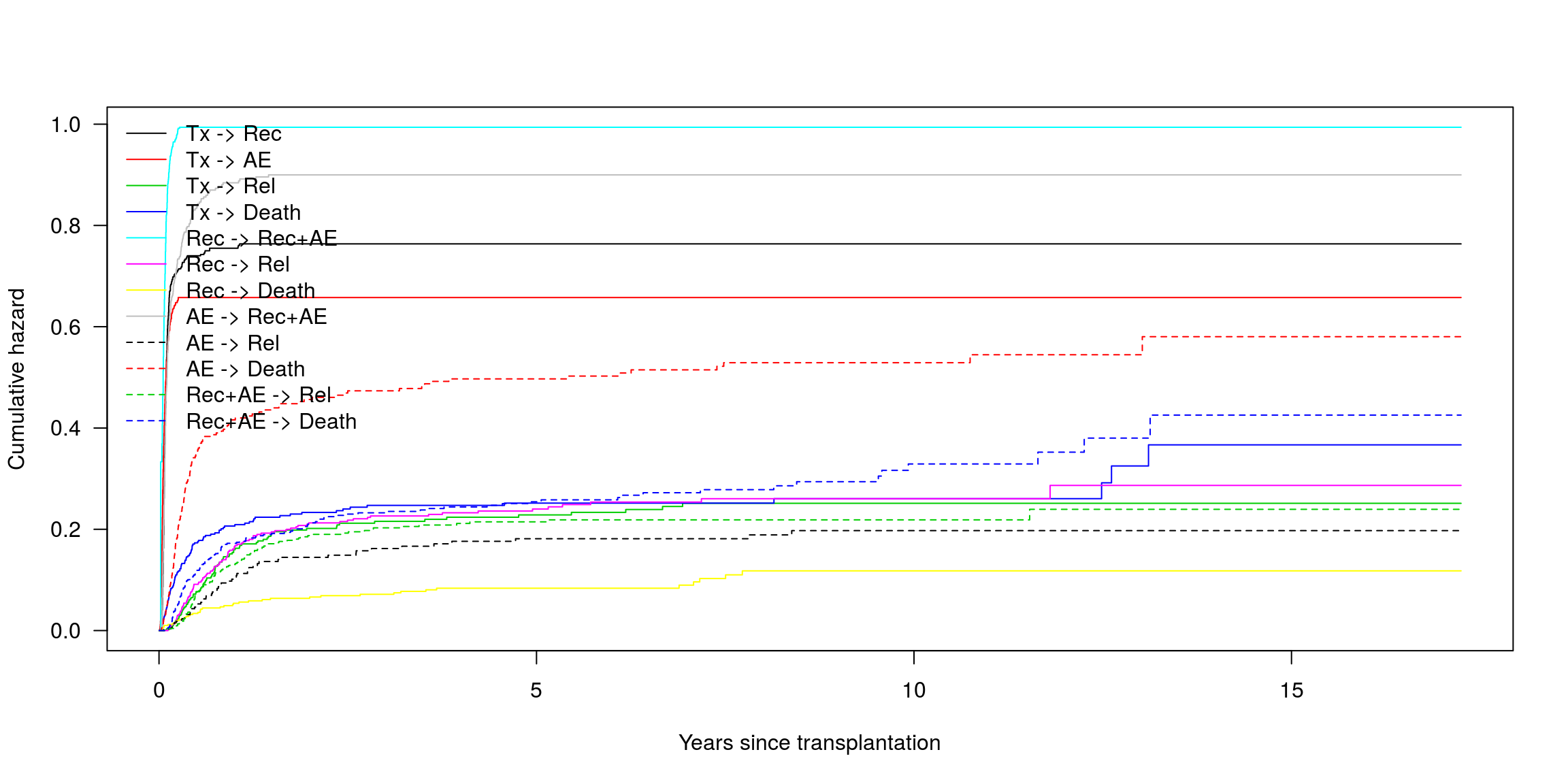
library(colorspace)
state_cols <- heat_hcl(6,
c = c(80, 30),
l= c(30, 90),
power = c(1/5,2))[6:1]
ord <- c(2, 4, 3, 5, 6, 1)
pt0 <- probtrans(msf0, predt = 0, method = "greenwood")
plot(pt0, ord = ord, las = 1, col = state_cols[ord],
xlab = "Years since transplantation", type = "filled")
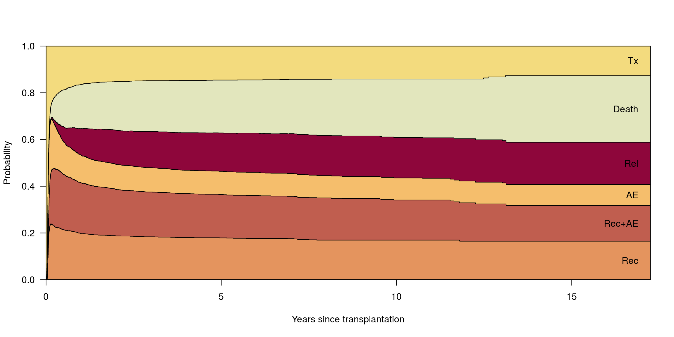
pt100 <- probtrans(msf0, predt = 100/365.25, method = "greenwood"); par(mfrow=c(1,2))
plot(pt100, ord = ord, xlim = c(0,10), las = 1, type = "filled", col = state_cols[ord], main = "Zaczynając od stanu 1")
plot(pt100, from = 3, ord = ord, xlim = c(0,10), las = 1, type = "filled", col = state_cols[ord], main = "Zaczynając od stanu 3")
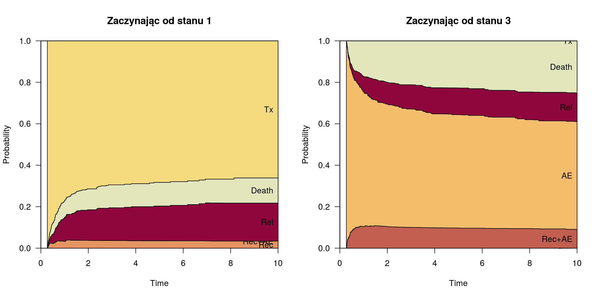
mvna
, etm
- także wspierają obliczenia skumulowanych hazardów
jednak nie mają wsparcia dla modeli semi-parametrycznych, jak model Coxa.
cfull <- coxph(Surv(Tstart, Tstop, status)~
match.1 + ... + match.12 +
+ proph.1 + ... + proph.12 +
+ ... + strata(trans), data = msebmt, method = "breslow")
Możliwe udoskonalenia
coxph
w postaci macierzy rzadkiejmsdata
do tworzenia nowych obserwacjiggplot2