Introduction

The metR package contains tools for comprehensive analysis of data from methylation studies. With the metR one can define regions, get basic statistics about methylation in them, plot methylation rate or rank these regions from the most interesting to the least one.

devtools::install_github("geneticsMiNIng/metR")
library(metR)
library(kableExtra)
library(knitr)

library(metR)

## Loading required package: ggplot2

## Loading required package: dplyr

## 
## Attaching package: 'dplyr'

## The following objects are masked from 'package:stats':
## 
##     filter, lag

## The following objects are masked from 'package:base':
## 
##     intersect, setdiff, setequal, union

## Loading required package: lme4

## Loading required package: Matrix

## Loading required package: nlme

## 
## Attaching package: 'nlme'

## The following object is masked from 'package:lme4':
## 
##     lmList

## The following object is masked from 'package:dplyr':
## 
##     collapse

## Loading required package: magrittr

## Loading required package: tidyr

## 
## Attaching package: 'tidyr'

## The following object is masked from 'package:magrittr':
## 
##     extract

## The following object is masked from 'package:Matrix':
## 
##     expand

## Loading required package: MASS

## 
## Attaching package: 'MASS'

## The following object is masked from 'package:dplyr':
## 
##     select

library(kableExtra)
library(knitr)

The data

Data for this example are downloaded from the site: http://www.neuroepigenomics.org/methylomedb/download.html. We used 4 control samples: Control1 AC, Control2 AC, Control3 AC and Control4 AC and 4 disease samples: SCZ1 AC, SCZ2 AC, SCZ3 AC, SCZ4 AC.

In the metR package these samples are available in the schizophrenia data frame. Each row is a single methylation probe. Data from all control/disease samples are combined together.

To speed up calculations and shrink down the size of data we are using only probes from chromosome 1. The R code needed to download data from all samples can be found in the script https://github.com/geneticsMiNIng/metR/blob/master/examples/prep.MethylomeDB.R. The result of this script is a single data.frame schizophrenia that is included in metR package. The last column category indicates if data are from control samples (‘control’) or from disease samples (‘disease’).

data('schizophrenia')

kable_styling(kable(head(schizophrenia, 4), "html", bootstrap_options = "striped" , full_width = T), position = "left",
font_size = 11) %>% row_spec(1:4, color = "black")

chr	poz	no	meth	unmeth	meth.rate	category
chr1	73465	6	1	5	0.1666667	control
chr1	73467	6	1	5	0.1666667	control
chr1	74406	10	5	5	0.5000000	control
chr1	74873	10	5	5	0.5000000	control

Process data

To obtain interesting regions in subsection Examples of differentially methylated regions we runned 4 functions from metR package:

preprocessing() - preprocessing schizophrenia data
create_tiles_max_gap() - creating regions
get_stats() - getting basin statistics about created regions
find_DMR() - ranking regions from the most interesting to the least one by different methods

Functions above are described in metR_step_by_step vignettes or in package documentation.

control <- schizophrenia %>% filter(category == 'control') %>%
  dplyr::select(-category)

disease <- schizophrenia %>% filter(category == 'disease') %>%
  dplyr::select(-category)

processed_schizophrenia <- preprocessing(control, disease)

tiles_schizophrenia <- create_tiles_max_gap(processed_schizophrenia, gaps.length = 100)

stats <- get_stats(tiles_schizophrenia)
data('find.DMR.results')
find.DMR.results$Reg.Log.Beta <- find.DMR.results$Reg.Log %>% filter(p.value < 0.001) %>% arrange(-abs(beta.coef))
find.DMR.results$Reg.Mixed.Beta <- find.DMR.results$Reg.Mixed %>% filter(p.value < 0.001) %>% arrange(-abs(beta.coef))
find.DMR.results$Reg.Corr.Mixed.Beta <- find.DMR.results$Reg.Corr.Mixed %>% filter(p.value < 0.001) %>% arrange(-abs(beta.coef))

top <- do.call(gdata::combine,lapply(find.DMR.results, metR::get_top, n = 100, stats = stats))

Examples of differentially methylated regions

Below we are presenting more advance example of comparison of results from different tests. We are showing 8 regions that are results of running metR package on schizophrenia data.

1. Region with maximum coverage

This region has the largest coverage from interesting areas. We have 394 observations. This region hasn’t huge methylation diff in two samples but this difference is stable along the entire length.

draw_show_table(which.max(top$meth.cov),top,processed_schizophrenia)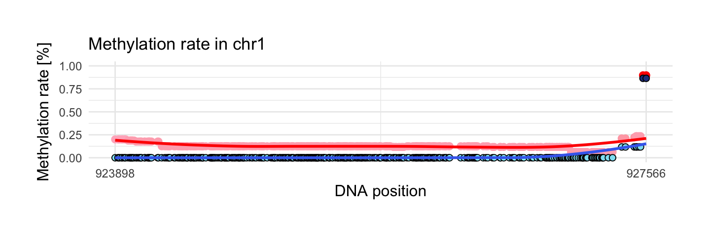

chr	start	end	meth.cov	meth.max_x	meth.max_y	meth.mean_x	meth.mean_y
chr1	923898	927566	394	0.9	0.86	0.13	0.01

meth.min_x	meth.min_y	meth.sd_x	meth.sd_y	meth.diff	quantile	source
0.06	0	0.06	0.06	0.12	0.94	Wilcoxon

2. Region with maximum mean of methylation rate in control sample

This region has the largest mean of methylation rate in control sample from interesting areas. We have 104 observations and mean of methylation rate is equal 1. This means that all of 104 observations have methylation rate on the level 1!

draw_show_table(which.max(top$meth.mean_x),top,processed_schizophrenia)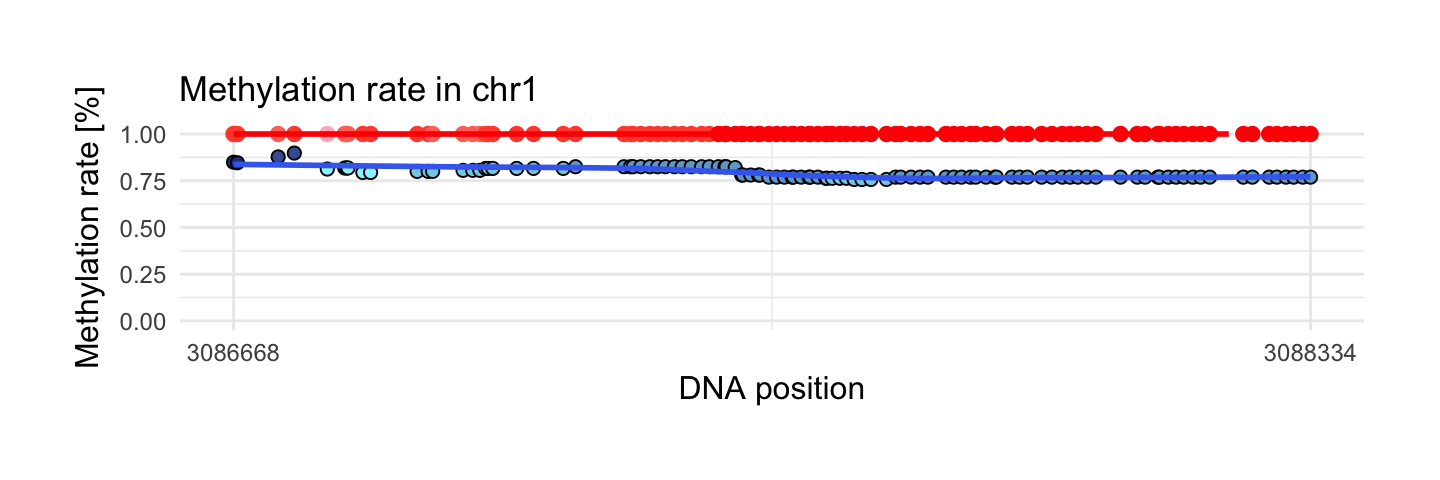

chr	start	end	meth.cov	meth.max_x	meth.max_y	meth.mean_x	meth.mean_y
chr1	3086668	3088334	104	1	0.9	1	0.79

meth.min_x	meth.min_y	meth.sd_x	meth.sd_y	meth.diff	quantile	source
1	0.76	0	0.03	0.21	0.98	Ttest

3. Region with minimum mean of methylation rate in disease sample

This region has the smallest mean of methylation rate in disease sample from interesting areas. We have 210 observations and mean of methylation rate is equal 0. This means that all of 210 observations have methylation rate on the level 0!

This is reverse example to the previous one.

draw_show_table(which.min(top$meth.mean_y),top,processed_schizophrenia)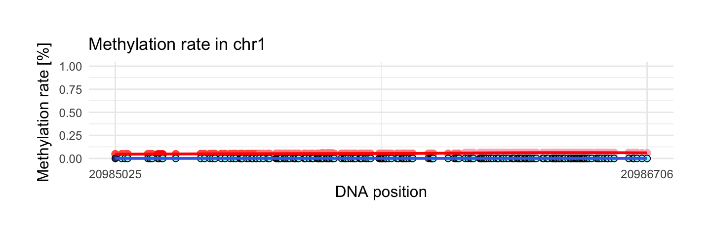

chr	start	end	meth.cov	meth.max_x	meth.max_y	meth.mean_x	meth.mean_y
chr1	20985025	20986706	210	0.06	0	0.06	0

meth.min_x	meth.min_y	meth.sd_x	meth.sd_y	meth.diff	quantile	source
0.05	0	0.01	0	0.06	0.85	Wilcoxon

4. Region with maximum standard deviation of methylation rate in control sample

We see very interesting regions below. In this example methylation rate start from 0 in both sample and increase to 1 in control sample and 0.75 in disease sample.

draw_show_table(which.max(top$meth.sd_x),top,processed_schizophrenia)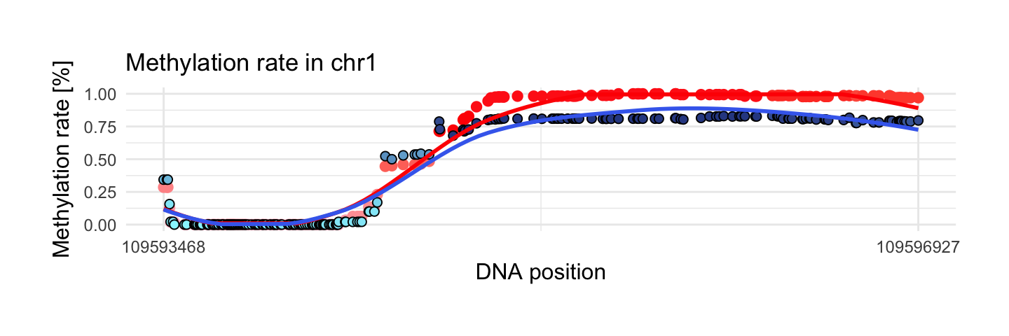

chr	start	end	meth.cov	meth.max_x	meth.max_y	meth.mean_x	meth.mean_y
chr1	109593468	109596927	223	1	0.83	0.42	0.36

meth.min_x	meth.min_y	meth.sd_x	meth.sd_y	meth.diff	quantile	source
0	0	0.47	0.39	0.07	0.87	Reg.Log

5. Region with maximum methylation difference in two probes

This area has only two observations but methylation difference between them is huge and equal 0.7.

draw_show_table(which.max(top$meth.diff),top,processed_schizophrenia)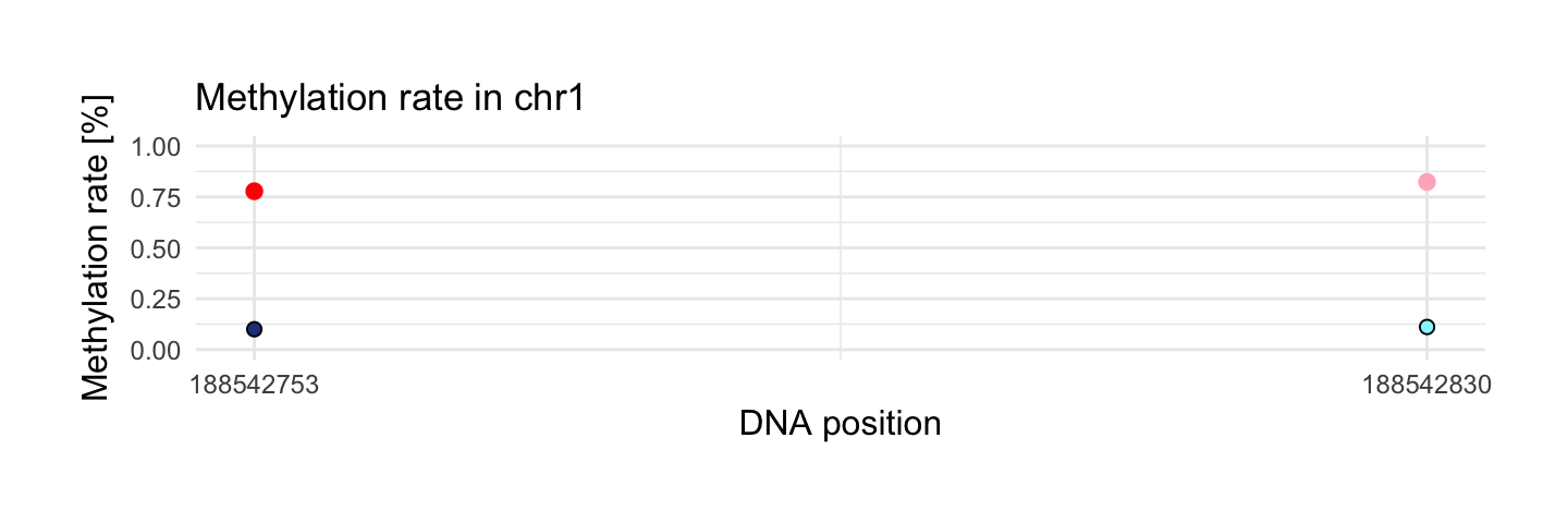

chr	start	end	meth.cov	meth.max_x	meth.max_y	meth.mean_x	meth.mean_y
chr1	188542753	188542830	2	0.82	0.11	0.8	0.11

meth.min_x	meth.min_y	meth.sd_x	meth.sd_y	meth.diff	quantile	source
0.78	0.1	0.03	0.01	0.7	1	Reg.Mixed.Beta

6. Region with maximum rank function

This area has maximum rank function. Rank function is based on quantile regression which uses information about number of observations in region. In this example methylation difference between probes is the biggest with respect to number of observations. Methylation difference is close to methylation difference in previous example but has more observation (11 to 2).

draw_show_table(which.max(top$quantile),top,processed_schizophrenia)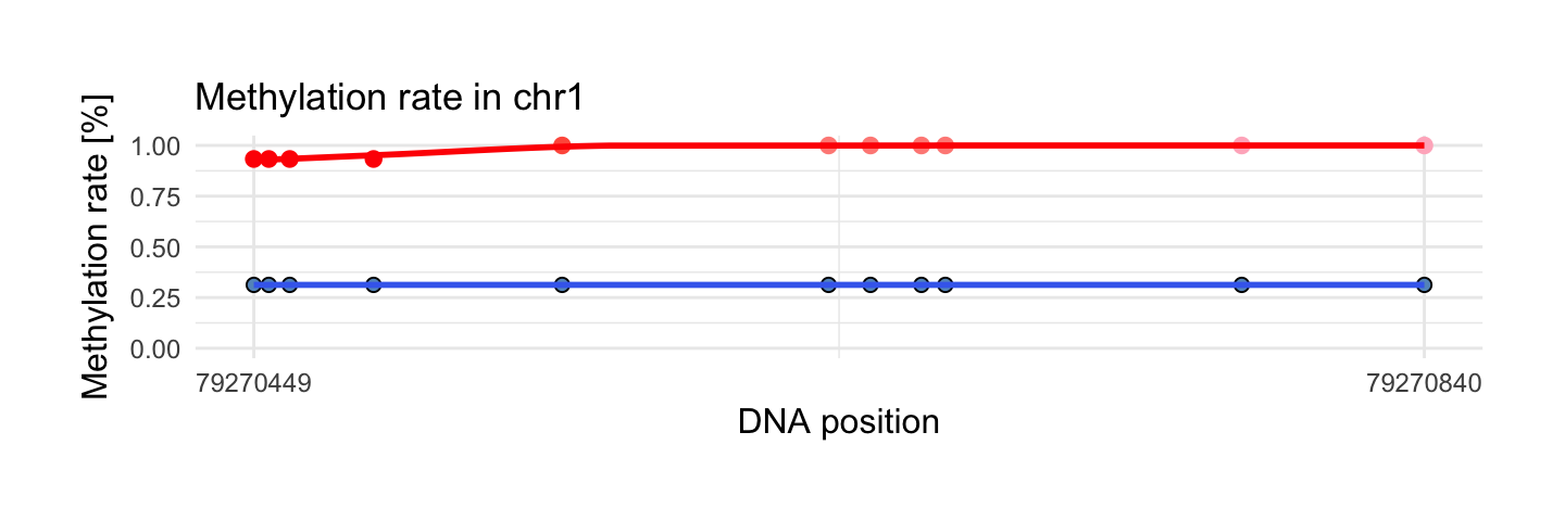

chr	start	end	meth.cov	meth.max_x	meth.max_y	meth.mean_x	meth.mean_y
chr1	79270449	79270840	11	1	0.31	0.98	0.31

meth.min_x	meth.min_y	meth.sd_x	meth.sd_y	meth.diff	quantile	source
0.93	0.31	0.03	0	0.66	1	Reg.Log.Beta

7. Region with maximum methylation range in control sample

This region has the biggest methylation range in control sample from interesting areas. We see that methylation rate in control sample starts from 1 and decreases to 0. In disease sample methylation rate starts from level 0.9 and decreases to 0.15. Curious observations is occurence that at the beginning of region we see bigger methylation in control sample and at the end of region reverse case.

draw_show_table(which.max(top$meth.max_x - top$meth.min_x),top,processed_schizophrenia)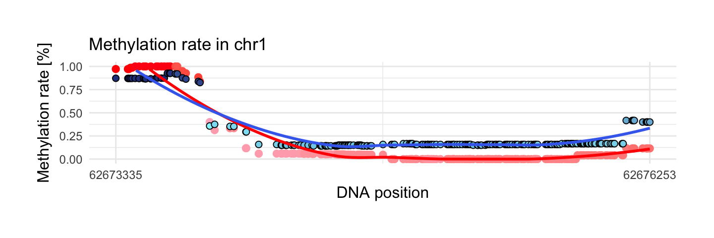

chr	start	end	meth.cov	meth.max_x	meth.max_y	meth.mean_x	meth.mean_y
chr1	62673335	62676253	233	1	0.93	0.13	0.25

meth.min_x	meth.min_y	meth.sd_x	meth.sd_y	meth.diff	quantile	source
0	0.14	0.29	0.22	0.12	0.93	Wilcoxon

8. Region with maximum methylation range in disease sample

This region has the biggest methylation range in disease sample from interesting areas. In the middle of region we can notice that methylation rate in disease sample is equal to 0 and in control is around 0.25. At the beginning and at the end of regions methylation increases in two probes.

draw_show_table(which.max(top$meth.max_y - top$meth.min_y),top,processed_schizophrenia)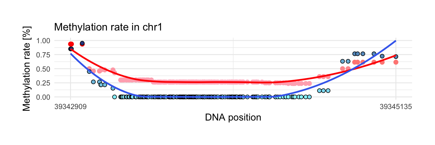

chr	start	end	meth.cov	meth.max_x	meth.max_y	meth.mean_x	meth.mean_y
chr1	39342909	39345135	177	0.94	0.95	0.3	0.06

meth.min_x	meth.min_y	meth.sd_x	meth.sd_y	meth.diff	quantile	source
0.24	0	0.12	0.19	0.24	0.99	Wilcoxon

Comparing all methods

Methods above are described in metR_step_by_step or in documentation find_DMR().

ggplot(top, aes(x = source, y = quantile)) + geom_boxplot(aes(fill = source))  + ggtitle('Distribution of rank rate by methods')  +
   scale_fill_brewer(palette = "Set1") + theme_minimal()  + theme(title = element_text(size = 14), axis.title = element_text(size = 13),
                           axis.text.y = element_text(size = 11), axis.text.x = element_text(size = 11, angle = 20) ,  legend.position = "None") +
  labs(x="Method",y="Rank rate") + 
  scale_x_discrete(limits=c('Reg.Mixed','Reg.Corr.Mixed.Beta','Reg.Corr.Mixed', 'KS', "Wilcoxon", 'Reg.Log.Beta', 'Reg.Mixed.Beta', 'Reg.Log', 'Ttest'))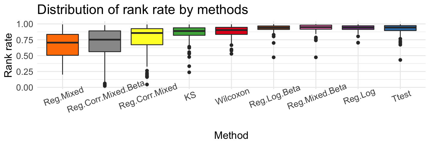

ggplot(top, aes(x = source, y = meth.diff)) + geom_boxplot(aes(fill = source))  + ggtitle('Distribution of methylation absolute difference by methods')  +
   scale_fill_brewer(palette = "Set1") + theme_minimal()  + theme(title = element_text(size = 14), axis.title = element_text(size = 13),
                           axis.text.y = element_text(size = 11), axis.text.x = element_text(size = 11, angle = 11) ,  legend.position = "None") +
  labs(x="Method",y="Methylation difference") + 
  scale_x_discrete(limits=c('Reg.Mixed','Reg.Corr.Mixed.Beta','Reg.Corr.Mixed', 'KS', "Wilcoxon", 'Ttest', 'Reg.Log', 'Reg.Log.Beta', 'Reg.Mixed.Beta'))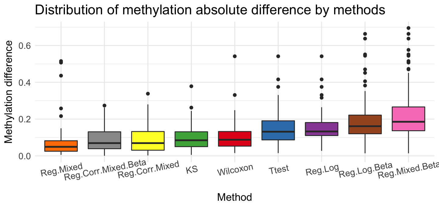

ggplot(top, aes(x = source, y = meth.cov)) + geom_boxplot(aes(fill = source))  + ggtitle('Coverage distribution by methods')  +
   scale_fill_brewer(palette = "Set1") + theme_minimal()  + theme(title = element_text(size = 14), axis.title = element_text(size = 13),
                           axis.text.y = element_text(size = 11), axis.text.x = element_text(size = 11, angle = 20) ,  legend.position = "None") +
  labs(x="Method",y="Coverage") + 
  scale_x_discrete(limits=c('Reg.Corr.Mixed.Beta','Reg.Log.Beta','Reg.Mixed.Beta', 'Reg.Mixed', "KS", 'Reg.Log', 'Reg.Corr.Mixed', 'Ttest', 'Wilcoxon'))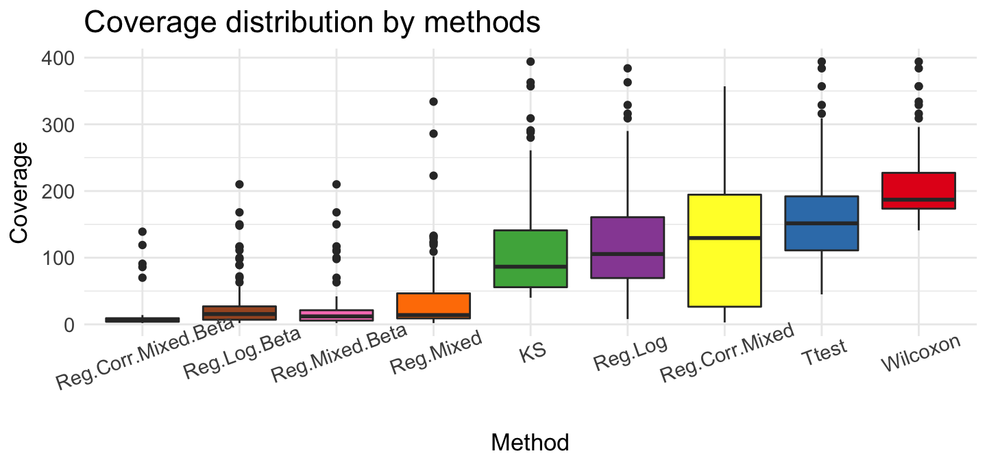

We can show, that these method given very different results. The rank rate is very good if we use Ttest, Reg.Log, Reg.Mixed.Beta and Reg.Log.Beta methods. The biggest differences we see for methylation coverage. Wilcoxon test recommended regions that have the most observations ~ 200. Reg.Corr.Mixed.Beta and Reg.Log.Beta proposed smaller group - about 10 observations. If we check methylation difference, Reg.Log.Beta and Reg.Mixed.Beta present very large difference in recommended regions.

Session info

devtools::session_info()

## Session info -------------------------------------------------------------

##  setting  value                       
##  version  R version 3.4.3 (2017-11-30)
##  system   x86_64, darwin15.6.0        
##  ui       X11                         
##  language (EN)                        
##  collate  en_US.UTF-8                 
##  tz       Europe/Warsaw               
##  date     2018-01-10

## Packages -----------------------------------------------------------------

##  package      * version date       source                        
##  assertthat     0.2.0   2017-04-11 CRAN (R 3.4.0)                
##  backports      1.1.1   2017-09-25 CRAN (R 3.4.2)                
##  base         * 3.4.3   2017-12-07 local                         
##  bindr          0.1     2016-11-13 CRAN (R 3.4.0)                
##  bindrcpp     * 0.2     2017-06-17 CRAN (R 3.4.0)                
##  colorspace     1.3-2   2016-12-14 CRAN (R 3.4.0)                
##  compiler       3.4.3   2017-12-07 local                         
##  datasets     * 3.4.3   2017-12-07 local                         
##  devtools       1.13.3  2017-08-02 CRAN (R 3.4.1)                
##  digest         0.6.13  2017-12-14 cran (@0.6.13)                
##  dplyr        * 0.7.4   2017-09-28 CRAN (R 3.4.2)                
##  evaluate       0.10.1  2017-06-24 CRAN (R 3.4.1)                
##  gdata          2.17.0  2015-07-04 CRAN (R 3.2.0)                
##  ggplot2      * 2.2.1   2016-12-30 CRAN (R 3.4.0)                
##  glue           1.1.1   2017-06-21 CRAN (R 3.4.1)                
##  graphics     * 3.4.3   2017-12-07 local                         
##  grDevices    * 3.4.3   2017-12-07 local                         
##  grid           3.4.3   2017-12-07 local                         
##  gtable         0.2.0   2016-02-26 CRAN (R 3.2.3)                
##  gtools         3.5.0   2015-05-29 CRAN (R 3.2.0)                
##  highr          0.6     2016-05-09 CRAN (R 3.4.0)                
##  hms            0.4.0   2017-11-23 cran (@0.4.0)                 
##  htmltools      0.3.6   2017-04-28 CRAN (R 3.4.0)                
##  httr           1.3.1   2017-08-20 CRAN (R 3.4.1)                
##  kableExtra   * 0.5.2   2017-09-15 cran (@0.5.2)                 
##  knitr        * 1.18    2017-12-27 cran (@1.18)                  
##  labeling       0.3     2014-08-23 CRAN (R 3.2.2)                
##  lattice        0.20-35 2017-03-25 CRAN (R 3.4.3)                
##  lazyeval       0.2.0   2016-06-12 CRAN (R 3.4.0)                
##  lme4         * 1.1-15  2017-12-21 cran (@1.1-15)                
##  magrittr     * 1.5     2014-11-22 CRAN (R 3.2.2)                
##  MASS         * 7.3-47  2017-02-26 CRAN (R 3.4.3)                
##  Matrix       * 1.2-12  2017-11-15 CRAN (R 3.4.2)                
##  memoise        1.1.0   2017-04-21 CRAN (R 3.4.0)                
##  methods      * 3.4.3   2017-12-07 local                         
##  metR         * 0.1.0   2018-01-09 local (geneticsMiNIng/metR@NA)
##  minqa          1.2.4   2014-10-09 CRAN (R 3.1.1)                
##  munsell        0.4.3   2016-02-13 CRAN (R 3.2.3)                
##  nlme         * 3.1-131 2017-02-06 CRAN (R 3.4.3)                
##  nloptr         1.0.4   2014-08-04 CRAN (R 3.2.2)                
##  pkgconfig      2.0.1   2017-03-21 CRAN (R 3.4.0)                
##  plyr           1.8.4   2016-06-08 CRAN (R 3.4.0)                
##  purrr          0.2.4   2017-10-18 cran (@0.2.4)                 
##  R6             2.2.2   2017-06-17 CRAN (R 3.4.0)                
##  RColorBrewer   1.1-2   2014-12-07 CRAN (R 3.2.2)                
##  Rcpp           0.12.14 2017-11-23 cran (@0.12.14)               
##  readr          1.1.1   2017-05-16 CRAN (R 3.4.0)                
##  rlang          0.1.6   2017-12-21 CRAN (R 3.4.3)                
##  rmarkdown      1.8     2017-11-17 cran (@1.8)                   
##  rprojroot      1.2     2017-01-16 CRAN (R 3.4.0)                
##  rvest          0.3.2   2016-06-17 CRAN (R 3.4.0)                
##  scales         0.5.0   2017-08-24 CRAN (R 3.4.1)                
##  splines        3.4.3   2017-12-07 local                         
##  stats        * 3.4.3   2017-12-07 local                         
##  stringi        1.1.6   2017-11-17 cran (@1.1.6)                 
##  stringr        1.2.0   2017-02-18 CRAN (R 3.4.0)                
##  tibble         1.3.4   2017-08-22 CRAN (R 3.4.1)                
##  tidyr        * 0.7.2   2017-10-16 cran (@0.7.2)                 
##  tidyselect     0.2.2   2017-10-10 cran (@0.2.2)                 
##  tools          3.4.3   2017-12-07 local                         
##  utils        * 3.4.3   2017-12-07 local                         
##  withr          2.1.0   2017-11-01 cran (@2.1.0)                 
##  xml2           1.1.1   2017-01-24 CRAN (R 3.4.0)                
##  yaml           2.1.16  2017-12-12 cran (@2.1.16)

metR: a deeper study

Aleksandra Brodecka

2018-01-10